Conducted Emissions in Power Supplies

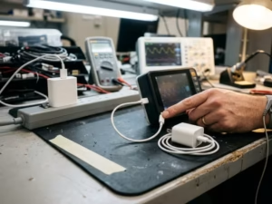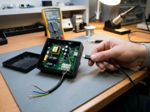
Your switching power supply looks clean on the bench. The output stays stable, and your quick scan shows nothing alarming.

Then the lab runs its conducted emissions sweep. Peaks jump over the limit line near 180 kHz and again at 600 kHz.

Conducted emissions are the noise currents a power supply pushes back onto its input lines. Labs measure them across a set range, usually 150 kHz to 30 MHz.

A failed scan costs you a retest, a redesign, and weeks of schedule.

I have debugged many of these failures. This guide shows you how to read the failure, what usually causes it, and which fixes work in real designs.

What Conducted Emissions Really Mean in a Power Supply

You don’t need a full EMC course to fix a conducted emissions failure. You do need three basics clear in your head. They shape every decision you make once the scan comes back red.

Conducted vs. Radiated Emissions

Radiated emissions travel through the air. The lab picks them up with an antenna, usually from 30 MHz upward.

Conducted emissions stay on the wires. Your power supply pushes noise current back onto its input lines, either the AC mains or a DC bus. The lab measures it right at that input, typically from 150 kHz to 30 MHz.

This article covers the second type: the noise your supply sends back down its own power cord. If you are comparing different product categories before test work starts, it helps to review the full range of power supply products.

Two Noise Modes, Two Different Fixes

Before you touch the filter, ask which way the noise travels. I ask this on every failure I debug.

Differential-mode (DM) noise flows out on one line and returns on the other. It mostly comes from ripple current in the input stage. You usually tame it with X-capacitors and series inductance.

Common-mode (CM) noise flows in the same direction on both lines. It returns through earth or chassis, often through stray capacitance you never drew on the schematic. You usually handle it with a common-mode choke, Y-capacitors, and less parasitic coupling.

A big X-capacitor does almost nothing for CM noise. A CM choke does little for DM noise. If you guess the mode wrong, you waste days.

How Engineers Measure It

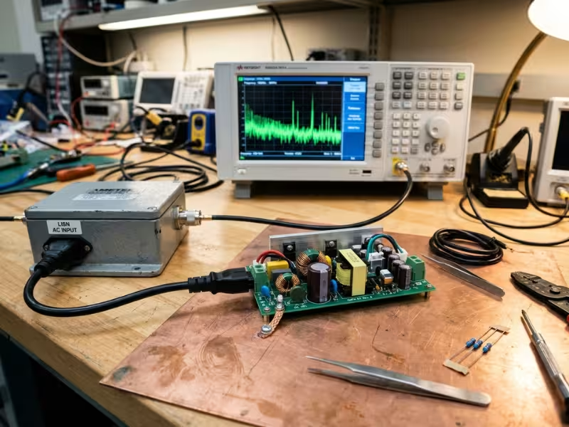
Every test starts with a LISN (Line Impedance Stabilization Network). It sits between the mains and your device. It gives your supply a fixed, repeatable source impedance, and it routes the noise to the measuring instrument.

An EMI receiver or a spectrum analyzer then reads that noise across the band.

Most standards set two limits:

• Quasi-peak weights noise by how often it repeats. It catches repeating bursts.
• Average sits about 10 dB lower. It catches steady tones, such as switching harmonics.

For quick bench scans, I use the peak detector. If the peak reading clears the average limit, you have nothing to worry about on either one.

How to Read a Conducted Emissions Failure Before You Start Fixing It

A failed scan feels urgent. Most teams grab a bigger choke or another capacitor within the hour.

I ask them to wait. The trace already tells you a lot about the cause. Ten minutes of reading it can save you a week of guesswork.

Start With the Trace, Not the Parts Drawer

First, mark your switching frequency on the plot. Then mark its multiples. A 65 kHz flyback puts harmonics at 130 kHz, 195 kHz, 260 kHz, and so on.

If the peaks line up with those marks, the switching stage drives the noise. Your job is to reduce the source or filter it harder.

Peaks that don’t line up point somewhere else. Each band gives its own clues:

• 150 kHz to about 2 MHz: Differential-mode noise usually dominates here. Input ripple current and weak DM filtering show up first.
• A broad hump in the low MHz range: This often means your input filter resonates. The filter amplifies noise near its own resonant frequency.
• Roughly 5 MHz to 30 MHz: Common-mode noise usually takes over. Look at stray capacitance from the switch node to the heatsink, chassis, or transformer.
• Sharp spikes at odd frequencies: Rectifier reverse recovery or snubber ringing often causes these.

These bands overlap, so treat them as leads, not verdicts. The next step confirms which mode you face.

Separate Common-Mode From Differential-Mode Early

I never change a filter part before I know the noise mode. A wrong guess sends you down the wrong path for days.

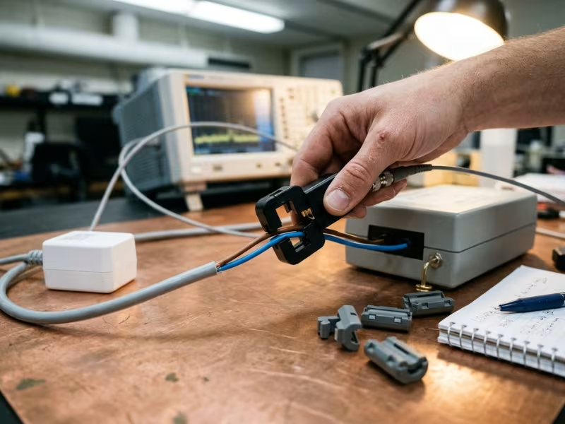
A current probe gives the fastest answer. Clamp it around both input wires together. The DM currents cancel, so the probe reads only CM noise. Then clamp one wire alone, or loop line and neutral through in opposite directions, to see the DM part.

Two quick bench tricks also help:

• Add a temporary X-capacitor across the input. If a peak drops sharply, it carries DM noise.
• Compare the LISN readings on line and neutral. Similar levels on both often point to CM noise.

A commercial DM/CM noise separator works well too, if your lab has one.

Test More Than One Operating Point

Many designs pass at one condition and fail at another. So I scan at four points: low line, high line, light load, and full load.

Each one shifts the noise in a different way:

• Low line raises input current, which pushes DM noise up.
• High line raises switch-node voltage swing, which pushes CM noise up.
• Light load can trigger burst mode or frequency foldback. That moves harmonics into new parts of the band.
• Full load increases ripple current through the input capacitors.

Quasi-resonant converters change frequency with both line and load. Their peaks move around the plot, so one scan rarely shows the full picture.

Mind the Gap Between Your Bench and the Lab

Pre-compliance scans work well, but they won’t match the certified lab exactly. Cable layout, ground plane size, LISN type, and receiver settings all shift the result. The quality of your setup, verification process, and hardware consistency also matters, which is why many teams review a supplier’s facilities before they commit to a platform.

I aim for at least 6 dB of margin on the bench. A 2 dB pass at your desk can turn into a fail on test day.

Pay extra attention to 150 kHz to 500 kHz. The limits drop steeply across this range. Your filter works least well at these low frequencies. And your strongest switching harmonics often sit right there. Many teams pass quasi-peak in this band but miss the average limit by a few dB.

The table below turns common trace patterns into first actions:

Where Conducted Emissions Usually Come From

When I open up a failing supply, I almost never find a mystery. The noise nearly always starts in one of five places. If you know these places, you can read your trace and go straight to the likely cause.

Fast Switching Edges Create the Raw Noise

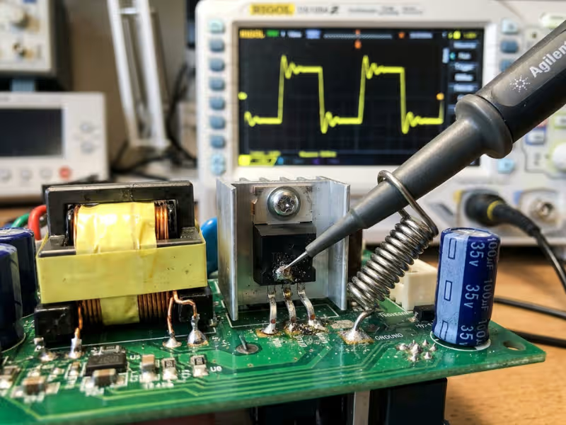
Every conducted emissions problem starts at the switch node. Each time your MOSFET turns on or off, the voltage on that node swings hundreds of volts in a few nanoseconds.

A typical silicon MOSFET switches at 10 to 30 V/ns. GaN and SiC devices can reach 50 to 100 V/ns. Faster edges mean higher efficiency, but they also push more energy into the upper part of the band.

A fast square wave holds a long chain of harmonics. Its spectrum stays strong up to a corner frequency set by the edge time, then rolls off. When you shorten the rise time, that corner moves higher. More of your noise then lands in the 5 to 30 MHz range.

The current edges matter too. Sharp di/dt in the switching loop creates voltage spikes across every nanohenry of trace inductance. Those spikes ring, and the ringing shows up as peaks on your scan.

Common-Mode Current Sneaks Through Parasitic Capacitance

The switch node doesn’t stay inside your circuit. It couples to anything nearby through stray capacitance.

Two paths cause most of the trouble:

• Switch node to heatsink or chassis. A TO-220 tab on an insulating pad can add 50 to 100 pF to a grounded heatsink.
• Transformer interwinding capacitance. The primary and secondary windings sit close together. They often form tens to hundreds of pF across the isolation barrier.

The numbers add up fast. At 20 V/ns, just 50 pF drives about 1 A of peak displacement current. That current flows to earth and comes back through the LISN as common-mode noise.

CM noise is hard to fix because its path doesn’t appear on your schematic. You can’t see it, and Y-capacitor limits restrict how hard you can filter it.

Differential-Mode Noise Follows the Input Current

DM noise comes from the current your converter actually draws. A flyback or forward converter pulls current in sharp pulses, not a smooth flow.

Your input capacitor tries to supply those pulses. But every real capacitor has ESR and ESL. The ripple current through them creates a ripple voltage, and that voltage appears on the line as DM noise.

Single-stage topologies make this worse. A flyback has discontinuous input current, so its harmonics start strong right at the switching frequency. A boost PFC stage running in continuous mode draws a much smoother current.

Rectifier reverse recovery adds sharp current spikes. A standard fast-recovery diode can dump a short burst of current every cycle. Those spikes create ringing and narrow peaks at odd frequencies.

A Poor Layout Can Sink a Good Design

I have seen two boards with the same schematic differ by 10 dB. The layout made all the difference.

Watch for these four problems:

• Large hot loops. The loop from the input capacitor through the switch and back acts like a small antenna and an inductor.
• Long return paths. Noise current takes a wide detour and couples into nearby traces.
• Poor placement. A filter placed far from the input connector lets noise bypass it.
• Line traces near the switch node. Noise couples straight into the input wiring after the filter.

That last one hurts the most. Your filter can work perfectly and still fail, because the noise jumps past it on the board.

Your Input Filter Can Make Things Worse

Many engineers assume more filtering always helps. It doesn’t.

Every LC filter has a resonant frequency. If the filter has little damping, it amplifies noise near that point instead of reducing it. You see a broad hump on the trace, often in the low MHz range.

The source impedance changes the picture too. The LISN presents roughly 50 Ω in parallel with 50 µH. Your converter’s input looks like a negative resistance to the filter. That interaction can raise the resonant peak and even unsettle the control loop.

So a filter that looked fine in simulation can fail on the bench. Always check its damping with the real source and load attached.

The table below sums up how each source tends to show up:

The Standards and Limits You Need to Confirm First

Many teams start tuning filters before they know which limit line they have to clear. That order wastes effort. Confirm three things first: which standard applies, which class you target, and which detector limits you must pass.

Start With Your Product Category

Your product’s market and use decide the standard, not your power supply topology. A 60 W adapter for a laptop and a 60 W supply for a PLC can face different rules.

Start by asking where the end product lives and what it powers. Then check the standard your customer or certification lab expects. If you sell a supply into someone else’s system, ask them which standard their product must meet.

If your product falls into the ITE and multimedia category, reviewing typical ITE power supply options can help you match the EMC target to the right form factor and application.

Class A vs. Class B Sets Your Design Target

Class A covers commercial and industrial settings. Class B covers homes and any place a product may end up near radios and TVs.

Class B limits sit much lower. Under CISPR 32, the Class B quasi-peak limit at 150 kHz is 66 dBµV. Class A allows 79 dBµV. That 13 dB gap can double the size of your input filter.

My rule is simple: if your product could reach a home, design for Class B from day one. Moving from Class A to Class B late usually means a new filter and sometimes a new board.

Why Quasi-Peak and Average Both Matter

Most standards check each frequency against two limits. The average limit sits about 10 dB below quasi-peak.

The two detectors react to noise in different ways:

• Steady switching harmonics read almost the same on both detectors. They usually fail the average limit first, because it sits lower.
• Bursty or intermittent noise reads high on quasi-peak but low on average. Burst mode at light load often fails quasi-peak while it passes average.

So a design can pass one limit and fail the other at the same frequency. Check both before you call a scan clean. If your bench peak reading already clears the average limit, you have room on both.

Fixes That Actually Reduce Conducted Emissions

Most teams treat conducted emissions as a filter problem. They add a bigger choke, scan again, and hope.

I work in a different order. First I quiet the source. Then I cut the path the noise takes. Then I filter what is left. Each layer makes the next one smaller, cheaper, and easier to tune.

Quiet the Source First

A dB you remove at the switch node is a dB you never have to filter. That is why I start here, even when the filter looks like the obvious suspect.

• Slow the gate drive a little. A larger gate resistor stretches the switching edge. Going from 10 Ω to 22 Ω often cuts dv/dt enough to drop high-frequency peaks by several dB. You pay with some switching loss, so check MOSFET temperature after the change. A split gate resistor with a diode lets you slow turn-off only, which usually helps the most.
• Add an RC snubber where the node rings. Ringing on the drain or across the output rectifier creates sharp peaks in the 5–30 MHz range. A small RC snubber, such as 100 pF to 470 pF with 10 Ω to 47 Ω, damps that ringing. Tune it on the bench while you watch the waveform, not just the scan.
• Clamp the flyback spike. Transformer leakage inductance throws a voltage spike at turn-off. An RCD clamp limits it and protects the MOSFET. A clean clamp also removes a lot of high-frequency energy.
• Pick the right rectifier. Hard-recovery diodes dump a current spike every cycle. Schottky diodes, soft-recovery parts, or SiC Schottky diodes in PFC stages remove most of that spike.
• Control the spectrum. Many controllers offer frequency jitter. It spreads each harmonic across a wider band, which lowers the reading on the receiver. I have seen jitter cut quasi-peak and average readings by 4–8 dB at low frequencies.

None of these fixes is free. But together they often save one full filter stage.

Cut the Coupling Path

Some noise will always exist at the switch node. The next goal is to stop it from reaching earth, chassis, or the secondary side. This is where most common-mode problems get solved.

• Shield the transformer. A shield winding between primary and secondary intercepts the capacitive current. Tie it to a quiet primary node, such as the bulk capacitor return. Some designers also add a small cancellation winding that injects opposite-phase current. On flyback adapters, a good shield can drop CM noise by 10 dB or more.
• Tie the heatsink to a quiet node. A heatsink bolted to the chassis turns the MOSFET tab into a CM antenna. If safety rules allow, connect the heatsink to the primary DC return instead. If it must stay grounded, use a thicker insulator or a shielded pad to cut capacitance.
• Give the noise a short way home. CM current needs a return path. A Y-capacitor from the secondary return to the primary bulk return gives it one. Keep that path short and direct. A long trace adds inductance and makes the capacitor useless above a few MHz.

Filter What Remains

Now the filter has a much smaller job. Size it for the noise that is left, not for the noise you started with.

• Place the DM corner frequency on purpose. A second-order LC filter rolls off at 40 dB per decade. If you need 40 dB of attenuation at 150 kHz, put the corner near 15 kHz. A corner set too high leaves the low band exposed.
• Choose the CM choke for your band. High-permeability MnZn ferrite works well in the low MHz range. Nanocrystalline cores give more impedance across a wider band. Check saturation at peak line current. Also note the choke’s leakage inductance. It gives you free DM inductance, which can let you shrink a separate DM inductor.
• Use X-capacitors for DM and Y-capacitors for CM. Pick safety-rated parts in both cases, usually X2 and Y1 or Y2.
• Respect the leakage budget. Every Y-capacitor leaks mains current to earth. A 2.2 nF Y-cap at 264 VAC and 60 Hz passes about 0.22 mA. Consumer safety standards allow only a few hundred microamps, and medical rules allow far less. Add up all your Y-capacitance before you add more.

Use Layout as Part of the Filter

A filter only works if the noise has to pass through it. Layout decides whether it does.

Keep the hot loop small. The input capacitor, switch, and transformer primary should sit close together with a tight return. Smaller loops radiate less and inject less noise onto nearby traces.

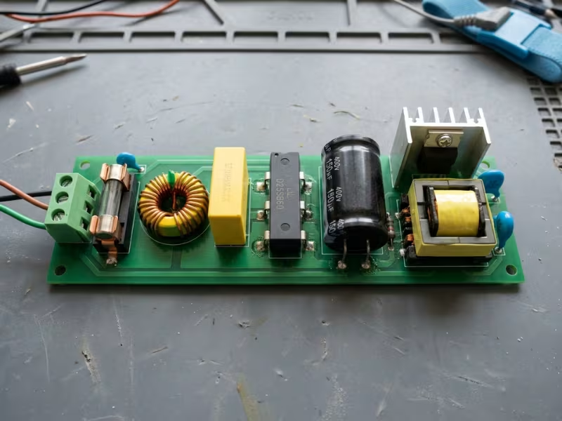
Follow a clean placement order: connector, fuse, CM choke, X-capacitor, bridge, bulk capacitor, switching stage. Keep the “dirty” side away from the “clean” input side. Never route input traces past the switch node.

Keep return paths tight under each current path. I have seen a layout fix cut emissions by 8 dB with no part changes. That gain often lets you remove a choke.

Retune or Add Another Stage?

When a scan still fails, the instinct is to add a second filter stage. Sometimes that is right. Often it is not the best first move.

Use this decision logic:

• Broad hump in the low MHz range? Your filter is probably resonating. Add damping, such as an RC damper across the filter capacitor, before you add anything else.
• Fail by 2–4 dB across a wide band? Retune the existing filter. Adjust inductance, capacitance, or the corner frequency.
• Fail above 10 MHz only? Check layout and coupling first. A small second CM choke may help, but parasitics often limit it.
• Need 15 dB or more at low frequency? A second stage makes sense. Damp both stages, and check that the filter does not upset your control loop.

A Real Debug Path: What to Change First When a Scan Fails

When a scan fails, the pressure to act fast pushes teams to change three parts at once. The peak drops, but nobody knows which change worked. Worse, one change may have helped while another hurt.

I follow the same six steps on every failure, and I change one thing at a time. A 45 W flyback adapter shows how this works. It failed CISPR 32 Class B by 5 dB at 390 kHz and by 8 dB near 18 MHz. The steps apply to almost any topology.

1. Confirm the band and the detector.
   Write down each failing frequency and which limit it broke. On the flyback, 390 kHz was the sixth harmonic of its 65 kHz switching frequency. It failed average but passed quasi-peak, which points to a steady switching harmonic. The 18 MHz peak failed both limits. That pattern usually means ringing or parasitic coupling.
2. Classify the noise mode.
   Clamp a current probe around line and neutral together. On the flyback, the 18 MHz peak stayed strong, so it was common-mode. The 390 kHz peak almost vanished, so it was differential-mode. That gave us two separate problems that needed two separate fixes.
3. Inspect the layout and cable path.
   Do this before you order parts. Check three things:
   On the flyback, the Y-cap return took a 40 mm detour. A short wire bodge cut the 18 MHz peak by 4 dB.
4. • Whether input traces run near the switch node
   • How long the Y-capacitor return path is
   • Whether the output cable lies across the transformer during the test
4. Test source-side fixes.
   Next, try to quiet the noise where it starts. We raised the gate resistor from 10 Ω to 22 Ω and added an RC snubber across the output diode. The 18 MHz peak dropped another 5 dB. The MOSFET ran 4 °C hotter, which stayed well inside its limits.
5. Retune the filter.
   Only now should you touch the filter. For the 390 kHz DM peak, we raised the X-capacitor from 100 nF to 220 nF. We also confirmed that the CM choke’s leakage inductance added useful DM filtering. The peak fell by 7 dB, and we never needed a second filter stage.
6. Re-scan with margin.
   Scan at low line, high line, light load, and full load, and check both detectors. Aim for 6 dB of margin at every point. The flyback finished with 6.5 dB at 390 kHz under its worst condition, low line, and 9 dB at 18 MHz.

Keep a simple log for every change. Record the part, the new value, the frequency it affected, and the dB shift. Take a photo of the cable layout too. When the certified lab result differs from your bench scan, that log shows you where to look first.

Common Mistakes and Trade-offs Engineers Underestimate

Most conducted emissions delays don’t come from hard physics. They come from fixes that look sensible on the bench and quietly create a new problem. I see these five again and again, and each one costs more the later you catch it.

Using a Bigger Filter to Hide a Layout Problem

The assumption: If the scan fails, the filter is too small. Add inductance or capacitance until the peak drops.

What happens: The peak drops a little, then stops moving. You add a second choke, and the 10–30 MHz band barely changes. The noise isn’t passing through the filter at all. It couples from the switch node into the input traces after the filter, or it rides a long Y-capacitor return. Meanwhile, the board gains cost, volume, and heat.

The better approach: Watch how the trace responds to each filter change. If a larger choke buys less than 2–3 dB, stop and look at the board. Shrink the hot loop, move input traces away from the switch node, and shorten the Y-cap return. A clean layout often lets you remove a filter part, not add one.

Ignoring Filter and Control-Loop Interaction

The assumption: The EMI filter and the converter are separate blocks. If each one works alone, they will work together.

What happens: A regulated converter draws constant power. As input voltage rises, input current falls, so the converter looks like a negative resistance to the filter. If the filter’s output impedance peaks near that value, the system can oscillate. You may see a low-frequency hum, an unstable output during line steps, or a new broad hump on the scan.

The better approach: Apply the Middlebrook criterion. Keep the filter’s output impedance well below the converter’s input impedance magnitude across the band. At low line and full load, that input impedance hits its lowest point, so check there first. Damp the filter with an RC branch across the filter capacitor, or add resistance in parallel with the inductor. Then verify with a line-step test, not just a scan.

Adding Too Much Y Capacitance

The assumption: Y-capacitors kill common-mode noise cheaply, so a few more nanofarads won’t hurt.

What happens: Emissions pass, and then the safety test fails. A 4.7 nF Y-cap at 264 VAC and 60 Hz passes about 0.47 mA to earth. A Class II adapter often has a touch-current budget in the low hundreds of microamps. Medical designs allow far less. One “small” fix can break your safety approval.

The better approach: Keep a running total of every Y-capacitor in the system, including any external inlet filter. Calculate leakage at maximum line voltage and frequency. When the budget runs tight, shift the work to a better CM choke, a transformer shield winding, or lower switch-node coupling.

Fixing Average While Creating a Quasi-Peak Failure

The assumption: The scan failed average, so you only need to watch the average limit.

What happens: A team enables a deeper burst mode at light load to cut steady harmonics. The average reading drops. But the bursts now repeat at a low rate, and the quasi-peak detector reads them high. The design trades one failure for another. Slow spread-spectrum modulation can cause a similar surprise.

The better approach: Re-scan with both detectors after every change. Repeat it at light load and full load. If a fix changes switching behavior, such as burst mode, jitter, or frequency foldback, treat it as a new design and check the whole band again.

Assuming Pre-Compliance Will Match the Certified Lab

The assumption: A pass on your bench means a pass at the lab.

What happens: The lab uses a different LISN, a larger ground plane, set cable lengths, and a calibrated receiver with a 9 kHz bandwidth. Your bench may use a spectrum analyzer with different settings and loose cables. Results often shift by 3–6 dB, and not always in your favor.

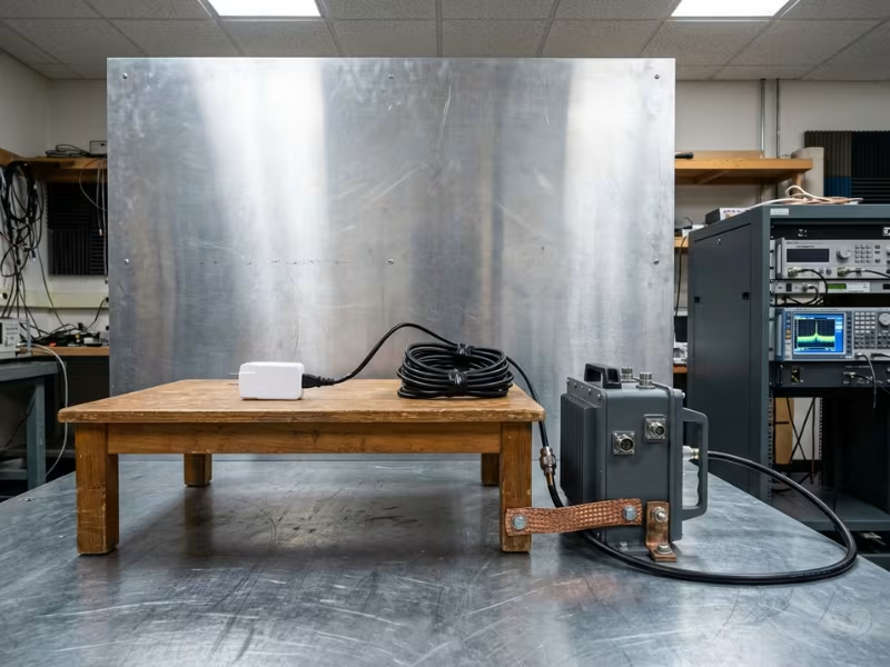
The better approach: Copy the lab setup as closely as you can. Place the unit 40 cm from a vertical ground plane, fold excess cable into a fixed bundle, and use the same cable you will ship. Keep 6 dB of margin. If you can, take one prototype to a lab early and compare its result with your bench scan. That single data point tells you how much to trust every scan after it.

A Practical Checklist Before You Book the Lab

A failed lab scan often means weeks of waiting for the next slot. I run through this list with every team before they book. Most items take an hour or less.

• Confirm the applicable standard.
  Ask your customer or lab which standard the end product must meet. CISPR 32, CISPR 11, and CISPR 25 set different limits and test setups. Write the answer down so the whole team designs to the same limit line.
• Lock in your Class A or Class B target.
  If the product could end up in a home, plan for Class B. The 13 dB gap at 150 kHz changes your filter size, so settle this before you pick any parts.
• Scan at four operating points.
  Test low line, high line, light load, and full load. Burst mode and frequency foldback can move peaks into new bands. Note which condition gives your worst result.
• Classify every failing peak as CM or DM.
  Clamp a current probe around line and neutral together, then around one wire. Label each peak on the plot. The label tells you whether you need a choke or an X-capacitor.
• Review the layout and hot loops.
  Keep input traces away from the switch node, and keep the hot loop tight. Measure the Y-capacitor return path. A short return often beats a bigger filter.
• Check the Y-capacitor leakage impact.
  Add up all Y-capacitance, including any inlet filter. Calculate leakage at maximum line voltage and frequency. Compare the total with your safety limit before you add more.
• Document margin, not just pass or fail.
  Log the dB margin at each critical frequency for both detectors. Aim for at least 6 dB. A 1 dB pass leaves no room for lab differences.
• Re-scan after every filter or layout change.
  One new part can push a peak up somewhere else in the band. Repeat the full sweep with both detectors at all four operating points. Save a photo of the cable layout with each result.

When every box has a tick and a number next to it, the lab confirms your work instead of surprising you.

FAQ

These six questions come up in nearly every design review I join. Here are the short answers I give engineers at the bench.

What frequency range does conducted emissions testing cover?

Most commercial standards test from 150 kHz to 30 MHz. That includes CISPR 32, CISPR 11, and FCC Part 15.

Other industries go higher. CISPR 25 for automotive extends the voltage method to 108 MHz. DO-160 for aerospace also reaches well past 30 MHz. Check your standard before you set your analyzer span. If you scan only to 30 MHz on an automotive design, you can miss a failure the lab will find.

What is the difference between Class A and Class B limits?

Class A covers commercial and industrial settings. Class B covers homes and anywhere near radios and TVs.

Class B is much stricter. Under CISPR 32 at 150 kHz, Class B allows 66 dBµV quasi-peak. Class A allows 79 dBµV. That 13 dB gap can double your filter size. If your product could reach a home, design for Class B from the start.

Why can a design pass quasi-peak but fail average?

The average limit sits about 10 dB below the quasi-peak limit. Steady switching harmonics read almost the same on both detectors. So they hit the lower average line first.

This happens most often between 150 kHz and 500 kHz, where your strongest harmonics sit. To fix it, add DM attenuation, adjust the X-capacitor, or move the switching frequency so a harmonic avoids the tightest region. Frequency jitter also helps. Re-check quasi-peak after any change to switching behavior.

How do I tell common-mode noise from differential-mode noise?

Use a current probe. Clamp it around line and neutral together. DM current cancels, so the probe reads only CM noise. Then clamp one wire alone to see the total.

For a quick bench check, add a temporary X-capacitor across the input. If a peak drops sharply, it carries DM noise. If it barely moves, suspect CM. As a rough guide, DM tends to dominate below 2 MHz, and CM tends to dominate above 5 MHz.

Do I need a LISN for pre-compliance testing?

Yes. Without a LISN, the mains impedance changes from outlet to outlet. Your readings won’t repeat, and they won’t compare with lab results.

A LISN gives your supply a fixed source impedance and routes the noise to your analyzer. Benchtop units cost far less than one failed lab slot. Add a transient limiter in front of your analyzer input. Power-up surges through the LISN can damage the analyzer’s front end.

How much margin should I leave before submitting to a certification lab?

I aim for at least 6 dB at every critical frequency, on both detectors. Check it across low line, high line, light load, and full load.

Raise that target if your units vary in production. Parts like Y-capacitors, chokes, and MOSFETs shift from batch to batch. Accept 3–4 dB only after you have correlated your bench setup with a real lab result. Without that data, a small margin is a gamble.

Fix the Source, Control the Path, Filter the Rest

Most conducted emissions failures don’t come from a filter that is too small. They come from fast edges, stray capacitance, and layout choices that push noise past the filter. A bigger choke can hide those problems for a while, but it rarely solves them.

So read the trace before you open the parts drawer. Mark the switching harmonics, find the failing band, and split common-mode from differential-mode with a current probe. That ten-minute check tells you whether you need a snubber, a shield winding, or an X-capacitor.

Then build margin early. A bench scan on your first prototype costs an afternoon. A late filter patch can cost a board respin, a new safety review, and a missed launch window.

Before you change one more part, scan at four operating points, label every peak CM or DM, and write down your margin on both detectors.